Exploring Random Forest Algorithm

Introduction

Random Forest is a popular supervised machine learning technique used for both regression and classification tasks. It stands out for its simplicity and effectiveness, often delivering excellent results without the need for extensive parameter tuning.

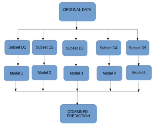
This algorithm works by creating multiple decision trees on different subsets of the data. Each tree makes its own prediction, and the final output is determined by combining the predictions of all the trees through a majority vote (for classification problems) or averaging (for regression tasks).

Here are some key points to understand about the Random Forest algorithm:

1. Ensemble Learning: Random Forest belongs to the ensemble learning category, where multiple models are combined to improve predictive performance.

2. Decision Trees: At its core, Random Forest builds decision trees. Each tree is constructed using a random subset of features and data points, making them diverse.

3. Voting Mechanism: For classification tasks, Random Forest aggregates the predictions of all individual trees and selects the class with the most votes as the final prediction.

4. Averaging: In regression tasks, the algorithm averages the predictions of all trees to produce the final regression estimate.

5. Robustness: Random Forest is less prone to overfitting compared to individual decision trees due to its ensemble nature and randomness in feature selection.

6. Scalability: It can handle large datasets with high dimensionality efficiently, making it suitable for real-world applications.

7. Feature Importance: Random Forest provides a measure of feature importance, which helps in understanding the contribution of each feature to the model's predictions.

8. Hyperparameters: While Random Forest typically performs well with default settings, there are hyperparameters that can be tuned to further optimize its performance, although it often works well without extensive tuning.

Ensemble Techniques

Suppose you want to purchase a house, will you just walk into society and purchase the very first house you see, or based on the advice of your broker will you buy a house? It’s highly unlikely.

You would likely browse a few web portals, checking for the area, number of bedrooms, facilities, price, etc. You will also probably ask your friends and colleagues for their opinion. In short, you wouldn’t directly reach a conclusion, but will instead make a decision considering the opinions of other people as well.

Ensemble techniques work in a similar manner, it simply combines multiple models. Thus, a collection of models is used to make predictions rather than an individual model and this will increase the overall performance. Let’s understand 2 main ensemble methods in Machine Learning:

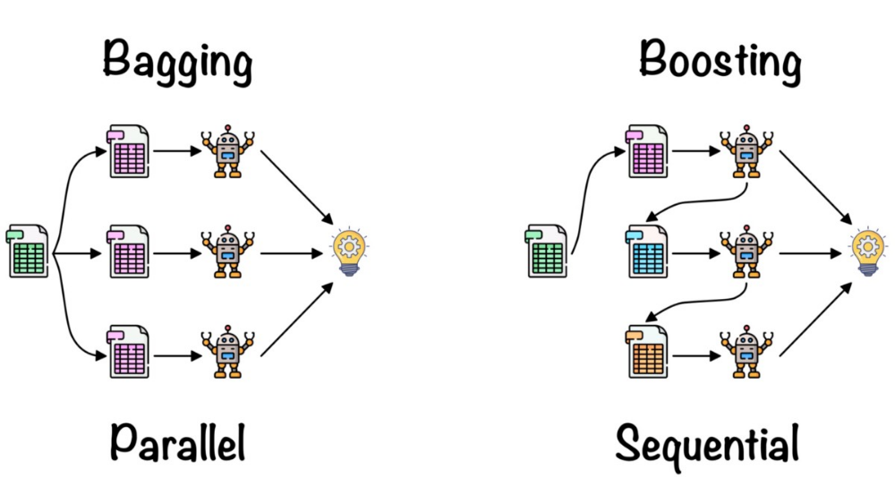
1. Bagging – Suppose we have a dataset, and we make different models on the same dataset and combine it, will it be useful? No right? There is a high chance we’ll get the same results since we are giving the same input. So instead we use a technique called bootstrapping. In this, we create subsets of the original dataset with replacement. The size of the subsets is the same as the size of the original set. Since we do this with replacement so there is a high chance that we provide different data points to our models.

2. Boosting – Suppose any data point in your observation has been incorrectly classified by your 1^st model, and then the next (probably all the models), will combine the predictions provide better results? Off-course it’s a big NO.

Boosting technique is a sequential process, where each model tries to correct the errors of the previous model. The succeeding models are dependent on the previous model.

It combines weak learners into strong learners by creating sequential models such that the final model has the highest accuracy. For example, ADA BOOST, XG BOOST.

Random forest works on the bagging principle and now let’s dive into this topic and learn more about how random forest works.

What is the Random Forest Algorithm?

Random Forest is a technique that uses ensemble learning, that combines many weak classifiers to provide solutions to complex problems.

As the name suggests random forest consists of many decision trees. Rather than depending on one tree it takes the prediction from each tree and based on the majority votes of predictions, predicts the final output.

Step-wise Procedure to Understand How Random Forest Works

Yes, it’s possible to understand the working of the random forest in 4 simple steps. But, before that, we need to understand one question about Random Forest.

Which type of ensembled learning random forest belongs to?

It belongs to bagging, where we build multiple decision trees called random forest.

Understanding random forests require a step-by-step approach. Here is a step-by-step guide.

Step 1: How a Complete Training Dataset is Used to Build Multiple Trees?

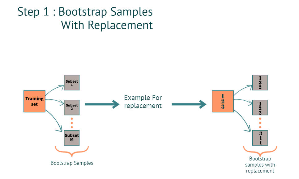
When we have a training dataset. The model creates a bootstrap sample with the replacement.

What is Bootstrap?

Creating multiple subsets from the actual training dataset.

How do we create multiple subsets when we have Rows and columns in the training dataset? and what is with replacement?

Rows:

When we say with thereplacement(refer to the image below for better understanding), in a subset, we can have the same row multiple times. as you can see in subset 2, the 2nd row is repeated 2 times, and in subset 3 1st row is repeated 2 times.

Columns:

1. For classification, it’s a square root of the total number of features

Example: let’s say we have a total of 4 features for each subset we will have

The square root of 4= 2. which is 2 features for each tree.

2. Regression: total number of features and dividing them by 3

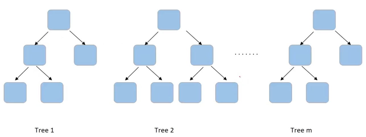
Step 2: Multiple Decision Trees can be Built by Following Steps

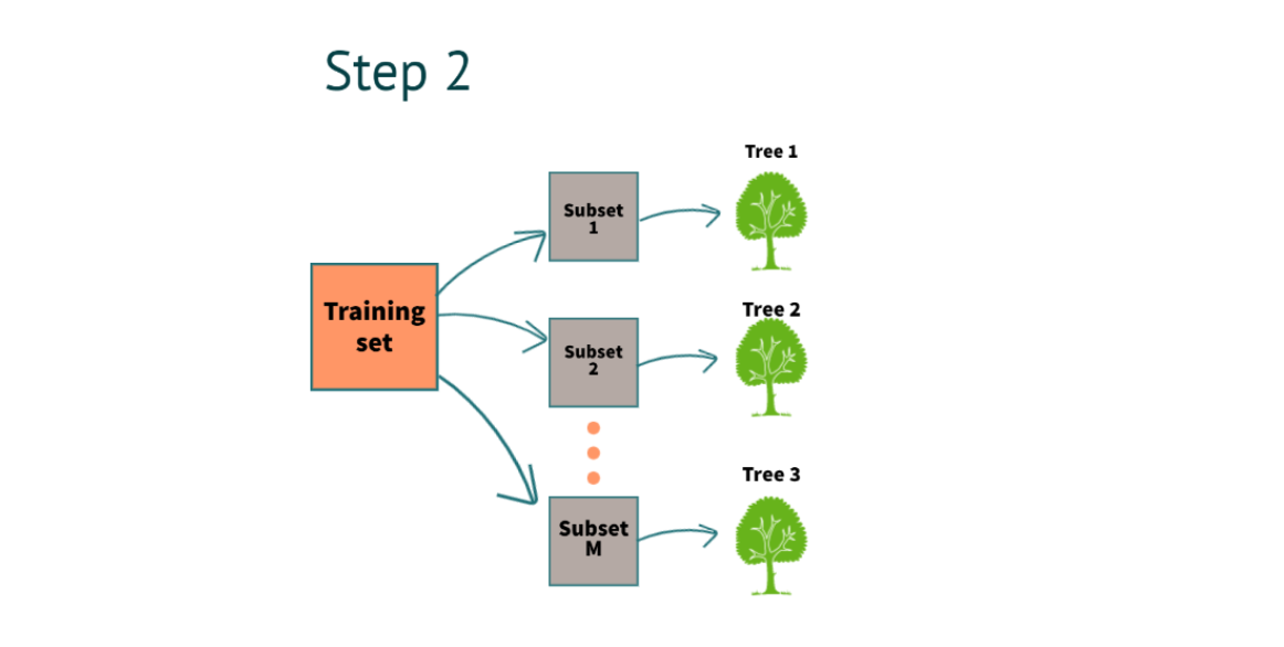
After completing step 1, we will build a decision tree for each subset. In the above example, we have 3 decision trees.

How were we able to build the decision trees from scratch?

To build a decision tree, we have to use two methods.

1. Gini

2. Entropy and Information gain

Step 3: Using Multi-tree Models for Predicting the Outcome, What is the Process of Predicting the Result?

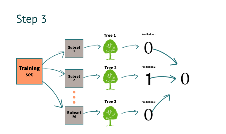
After building the decision tree now, it’s time to get the results. suppose we have new information for prediction

The model predicts it as “0”. By combing all decision tree predictions above, as you can see in the image

What do we mean by combining the prediction of all the trees?

To understand it, we go to step four.

Step 4: When a Model Finalizes a Result for Regression or Classification, What is it Called?

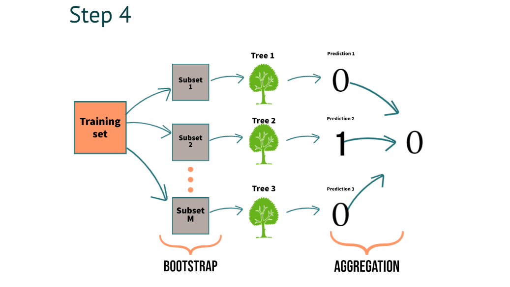
In Step 4, we can clearly understand the process of combining the predictions of multiple trees we call aggregation

1. For classification, we use majority voting

2. For regression, we use averaging

with this, we understand what exactly a bootstrap aggregation is all about.

Now, We need to understand how it benefits.

It reduces the variance. This helps build robust models, which work well even on unseen data.

Hyper-parameters of Random Forest

First, understand what the term hyper-parameters means? We have seen that there are multiple factors that can be used to define the random forest model. For instance, the maximum number of features used to split a node or the number of trees in the forest. We can manually set and tune these values. So I can set the number of trees to be 20 or 200 or 500. We can manually change and update these values. And these are called the hyper-parameters of random forest.

1. n_estimators: Number of trees

Let us see what are hyperparameters that we can tune in the random forest model. As we have already discussed a random forest has multiple trees and we can set the number of trees we need in the random forest. This is done using a hyperparameter “n_estimators”

2. max_features

There are multiple other hyper-parameters that we can set at a tree level. So consider this one tree in the forest-

Can you think of hyper-parameters for this tree? Firstly, if we can set the number of features to take into account at each node for splitting, for example-

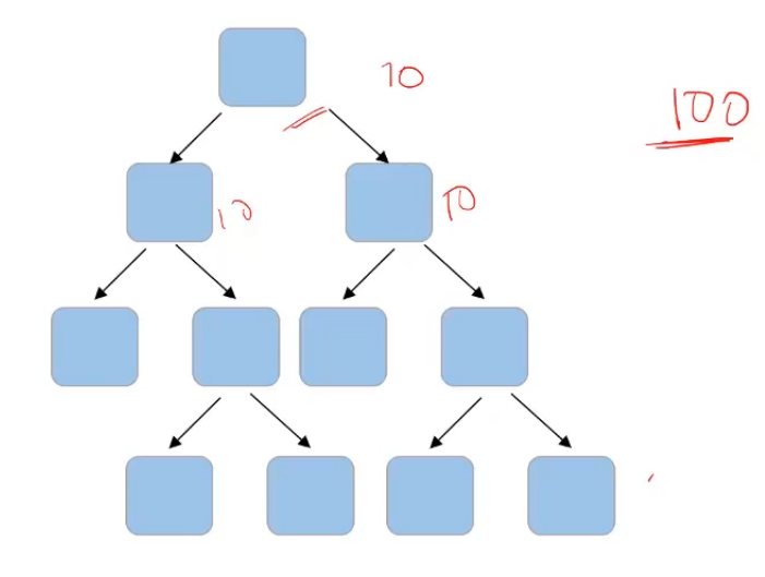
If the total number of features in my data set is a hundred and I decide that I’ll randomly select the square root of these total number of features. So which comes out to be 10. So I’ll randomly select 10 features for this node and the best feature will be used to make the split. Then again, I’ll randomly select 10 features for another node. And similarly, for all the nodes, instead of taking a square root, I can also consider taking the log of the total number of features in the dataset. So “max_features” is one of the parameters that we can tune to randomly select the number of features at each node.

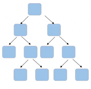
3. max_depth

Another hyperparameter could be the depth of the tree. For example, in this given tree here,

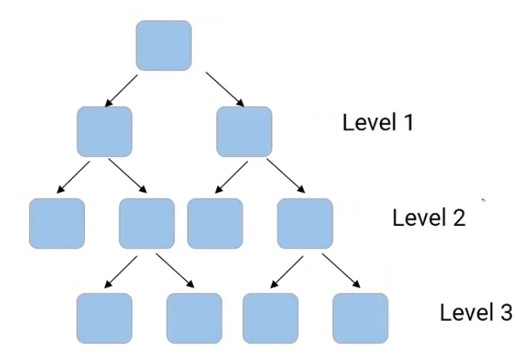
we have level one, we have level two, and a level three. So the depth of the tree, in this case, is three. We can decide the depth to which a tree can grow using “max_depth“, and this can be considered as one of the stopping criteria that restrict the growth of the tree.

4. min_samples_split

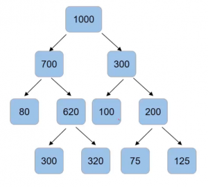
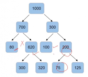
Another value that we can control is the minimum number of samples required to split a node and the minimum number of samples at the leaf node. So for instance, if I have a thousand data points and after the first split, I have 70o in one node and 300 in the other node. And here are the values of the number of data points in each of the node after splitting-

Now we can set the criteria that a normal split only when the number of samples in the node is more than 100 using “min_samples_split“. So node with 80 samples will not have for the split, same as the case with a node with 100 and 75 samples since our condition is that the number of samples should be more than 100.

5. min_samples_leaf

Another condition that we can set is the number of samples in the leaf node using “min_samples_leaf“. So if I save that the split can happen only when after the split, the number of samples in the leaf node comes out to be more than 85. Then, in that case, this will be an invalid split since, after the split, the number of samples is only 80-

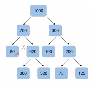
The split on 300 and 620 are valid but the split on 200 will not take place-

6. criteria

Another important hyper-parameter is “criteria“. While deciding a split in decision trees, we have several criteria such as Gini impurity, information gain, chi-square, etc. Similarly, we can have some other criteria like entropy. So to set, which criteria to use will be done using the hyperparameter “criteria”.

So these were the most important hyper-parameters of random forest.

Python Implementation

# Importing the necessary libraries
import pandas as pd
import numpy as np
from sklearn.datasets import load_iris
data = load_iris()

load the iris dataset from the sklearn library

# Convert the iris data into a Pandas data frame with feature names as column names
df = pd.DataFrame(data.data, columns=data.feature_names)

# Add a new column 'target' to the dataframe using target names and target codes
df['target'] = pd.Categorical.from_codes(data.target, data.target_names)
# Print first 5 rows of the dataframe
print(df.head())

We’re printing the first 5 rows after converting the data into a data frame.

# Split the data X and y 
X = df.drop('target',axis=1)
y = df['target']

# Import train_test_split function from sklearn
from sklearn.model_selection import train_test_split

X_train, X_test, y_train, y_test = train_test_split(X, y, test_size=0.3, random_state=0)

# Import the RandomForestClassifier from sklearn
from sklearn.ensemble import RandomForestClassifier

classifier_rf = RandomForestClassifier(random_state=42, n_jobs=-1, n_estimators=20)

We are using a random forest classifier with Hyper parameter

1. Random_state(it helps to generate the same results every we run the model)

2. n_jobs ( it uses all the processors)

3. n_estimators( we are using 20 decision tree in the random forest. if we want, we can tune it.

# Fit the training data
classifier_rf.fit(X_train, y_train)
# Predict on testing data 
y_pred = classifier_rf.predict(X_test)

from sklearn.metrics import confusion_matrix, classification_report, accuracy_score
print(confusion_matrix(y_test, y_pred))
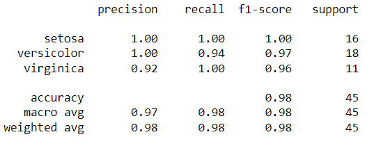
print(classification_report(y_test, y_pred))

We have the predictions saved in the y_pred variable. We can compare the actual vs. predicted using the report below.

Conclusion

In this article, we looked at the most popular algorithm. To summarize, we learned about Random Forest in detail. Let’s take a look at the key takeaways.

Key takeaways:

1. Random forest gives us better accuracy than the single decision tree because the information will be passed to multiple trees.

2. In real-time, we don’t get balanced datasets, and because of that, most of the machine learning models will be biased toward one specific class. Still, Random forest can handle an imbalanced dataset by randomizing the data.

3. We use multiple decision trees to average the missing information. So, with Random forest, we can also handle the missing values.

4. Lastly, It helps to build robust models in real-time by reducing variance.